Understanding Quantization in Deep Learning
Understanding Memory Footprint
When working with deep learning models, understanding memory usage is crucial. The total memory consumption can be broken down into two main components:
Example: Calculating Model Memory
Memory Optimization Techniques
Let's explore key techniques for reducing memory usage in deep learning models, starting with an important but often overlooked approach:
1. Gradient Checkpointing
Gradient checkpointing is a powerful technique that trades computation time for memory savings. Instead of storing all activations in memory during the forward pass, we do the following:
Strategy:
- Store activations at checkpoints only
- Recompute intermediate activations when needed
- Free memory after gradients are computed
Trade-offs:
- ✓ Reduced memory footprint
- ✗ Increased training time (recomputation)
Basics and Lookup Table
Understanding INT4 Range
When we say INT4 (4-bit integer) has a range of -8 to 7, we're describing the minimum and maximum values that can be represented using 4 bits in signed integer format. Let's break this down:
- Signed integers reserve one bit for the sign (positive/negative)
- Two's Complement allows efficient hardware implementation
- The range is asymmetric around zero (-8 to +7) due to Two's Complement
2. Understanding Quantization
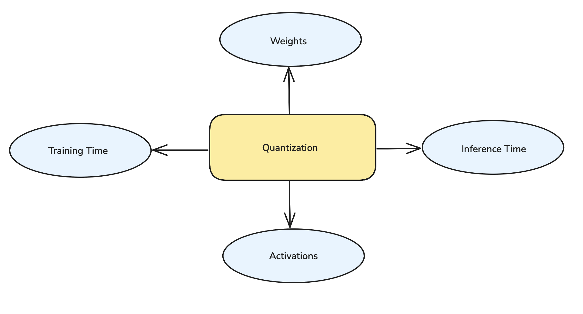
From the figure, we now understand that:
- Quantization can be applied to weights, Activations.
- It can also be applied in Inference time and Training time.
Let's see one by one.
1. Quantizing Weights (Static and Stable)
Weights are ideal candidates for quantization because they change less frequently. Once trained, weights remain constant unless the model is fine-tuned, making them perfect for one-time quantization.
| Original Weight | Quantized Value (INT8) |
|---|---|
| 0.45 | 92 |
| -0.23 | 35 |
| 0.89 | 127 |
| -0.75 | -128 |
- Weights only need to be quantized once after training
- Quantized model can be used repeatedly without re-quantization
- More predictable impact on model performance
2. Quantizing Activations (Dynamic Values)
Unlike weights, activations change with every inference because they depend on the input data. This makes activation quantization more challenging and requires careful consideration of the dynamic range.
- Dynamic range varies with each input
- Requires runtime quantization/dequantization
- May need batch-wise statistics for better accuracy
- More sensitive to quantization errors than weights
Inference Time Quantization
Inference time quantization focuses on serving the model in low precision to accelerate computation. Modern approaches have moved beyond simple quantization to mixed precision strategies, which offer a better balance between performance and accuracy.
In a typical mixed precision setup:
- Model weights are stored in FP16 or FP8 format for memory efficiency
- Activations and gradients use FP32 or FP16 for better numerical stability
- Critical operations may dynamically switch between precisions as needed
Quantization-Aware Training (QAT)
QAT is a training-time technique designed to maintain high accuracy when models are deployed with low-bit quantization (like INT8, INT4). Unlike post-training quantization, QAT allows the model to adapt to quantization effects during the training process itself.
How QAT Works
The QAT process involves four key steps:
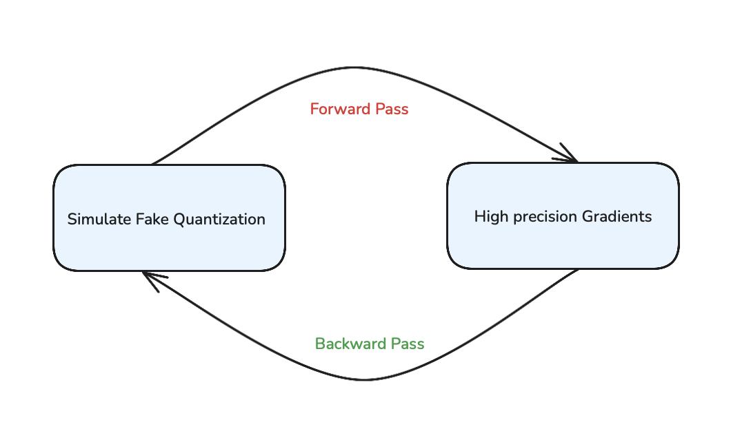
1. Simulate Quantization During Training
During the forward pass, weights and activations are "fake quantized" to simulate deployment conditions. This involves rounding and clipping values based on the target precision (like INT8), helping the model learn to work within quantization constraints.
2. Backpropagate Using High Precision
The backward pass maintains high-precision gradients (typically FP32) to ensure accurate learning. This dual approach allows stable gradient updates while still preparing the model for quantized deployment.
- The model adapts during training to minimize the accuracy loss that might occur from quantization
- It learns to "expect" the noise from quantization and adjusts accordingly
- Once training is complete, the model weights are actually quantized to low-bit precision for deployment
Common Challenges
When implementing QAT, teams typically face several challenges:
- Balancing training time with quantization accuracy
- Choosing appropriate quantization parameters
- Handling layers with different sensitivity to quantization
- Managing the increased complexity of the training pipeline
What's Next?
In our next article, we'll explore advanced memory-efficient techniques like LoRA (Low-Rank Adaptation) and other parameter-efficient fine-tuning methods that are revolutionizing how we train large language models.
Did you find this article helpful? Have questions about implementing these techniques? I'd love to hear your thoughts and experiences in the comments below! Your feedback helps make these explanations better for everyone.