GPU Fundamentals & LLM Inference Mental Models
Research Engineer interviews at leading AI labs test your ability to reason about inference performance from first principles. You will be expected to estimate whether a model fits on a given GPU, explain why autoregressive decoding is slow, identify bottlenecks (memory bandwidth vs. compute) for a given workload, and propose optimizations that target the actual bottleneck.
This article builds that foundation. We cover GPU architecture, the roofline model, memory estimation, arithmetic intensity analysis, and latency estimation , everything you need to develop strong intuition about what makes LLM inference fast or slow.
GPU Architecture Fundamentals
NVIDIA A100 Architecture
The A100 is the workhorse GPU for LLM inference and training. Understanding its architecture is essential for reasoning about performance.
The A100-80GB packs 108 SMs, each with 64 CUDA cores and 4 Tensor cores, connected via 40 MB L2 to 80 GB HBM2e at 2 TB/s. Fast on-chip SRAM (192 KB per SM) sits next to each SM; the size and speed gap between SRAM and HBM is what makes memory bandwidth the bottleneck.
Key Numbers to Memorize
Execution Model: Warps and Thread Blocks
- Kernel launch → a grid of thread blocks is scheduled onto SMs.
- Each block has up to 1024 threads, split into warps.
- Each warp = 32 threads executing in lockstep (SIMT); they all run the same instruction at once.
The warp is the fundamental unit of execution. All 32 threads in a warp execute the same
instruction at the same time. If threads diverge (different if branches), both paths must be
executed serially , this is called warp divergence and it wastes cycles.
SRAM vs. HBM: The Crucial Ratio
- Total SRAM: ~20 MB (fast, on-chip, ~30 cycle latency)
- Total HBM: 80 GB (slow, off-chip, ~400 cycle latency)
- Ratio: HBM is ~4000x larger but ~13x slower
This mismatch is the fundamental reason why memory bandwidth is the bottleneck for most LLM inference workloads. The model weights live in HBM, and for each token generated during decode, we must read ALL weights from HBM through a limited bandwidth pipe.
Memory Hierarchy Latency
Why This Matters for LLM Inference
During autoregressive decode, each generated token requires reading the full model weights from HBM:
- Llama-7B at FP16: 14 GB of weights
- At 2 TB/s bandwidth: Takes 14 GB / 2 TB/s = 7 ms just to read the weights
- Computation: ~14 GFLOP per token, which at 312 TFLOPS takes only 0.045 ms
The weight-loading time is 150x larger than the compute time. This is why decode is memory-bandwidth-bound, and why all the major inference optimizations (quantization, KV caching, speculative decoding, batching) ultimately aim to reduce the bytes-per-useful-FLOP ratio.
The Roofline Model
The roofline model is the single most important mental model for understanding inference performance. It tells you whether a workload is limited by:
- Memory bandwidth (loading data from HBM) , left side of the plot
- Compute throughput (doing arithmetic) , right side / top of the plot
Arithmetic Intensity
Ridge Point
The ridge point is the arithmetic intensity at which the compute and memory roofs intersect:
Attainable Performance
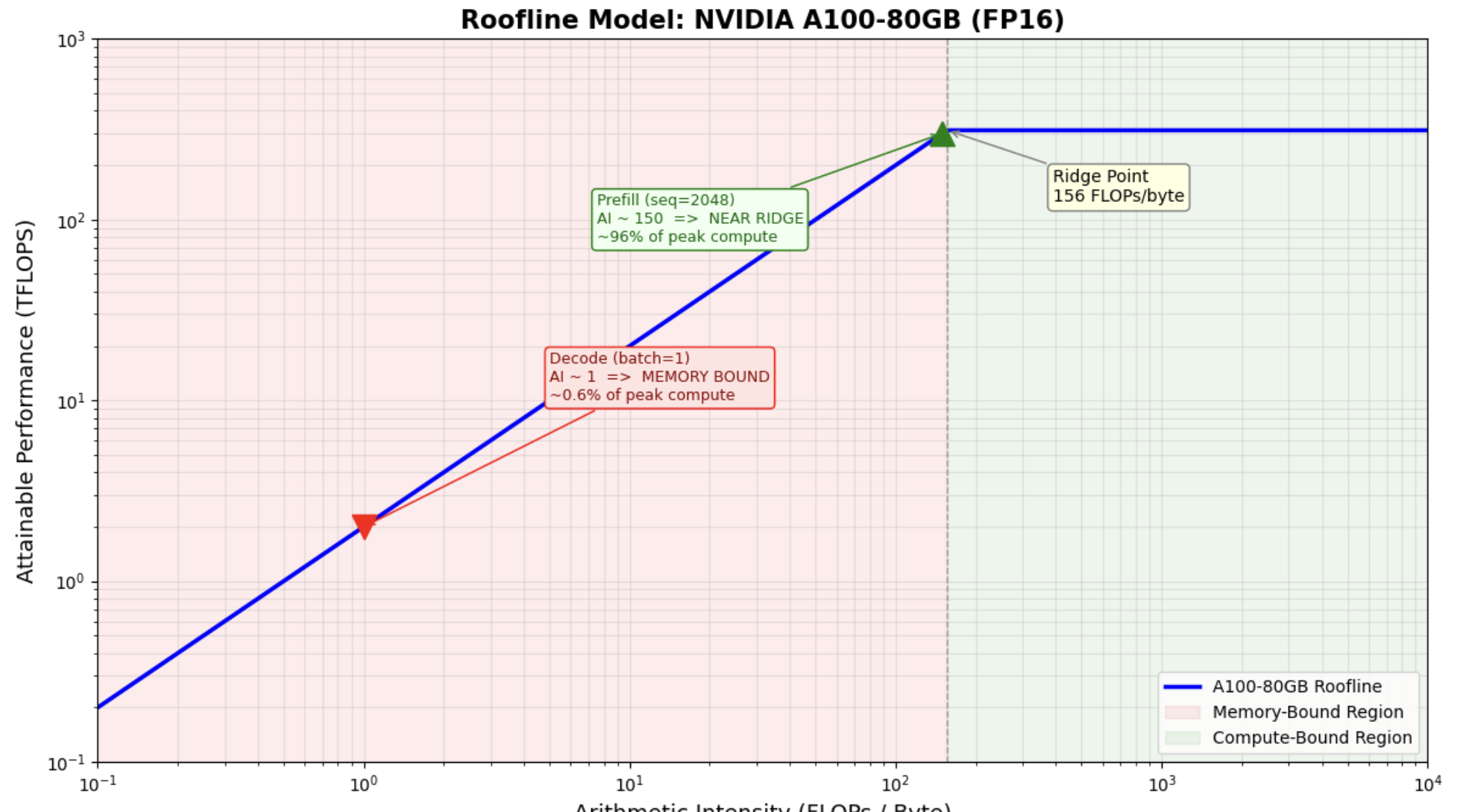
The Key Insight: Prefill is Compute-Bound, Decode is Memory-Bound
This single insight explains nearly every optimization in modern LLM serving.
Prefill
Decode
Why is decode so memory-inefficient? During decode, we generate ONE token. This means we
do a matrix-vector product: the weight matrix has d_model × d_model elements, but the
input vector has only d_model elements. Each weight is loaded from HBM but used for only
one multiply-add (2 FLOPs / 2 bytes at FP16 = AI of 1).
Why is prefill efficient? During prefill, the input is a matrix of shape
(seq_len × d_model). The same weight matrix (loaded once from HBM) is multiplied
against seq_len vectors. The weight bytes are amortized across
seq_len tokens, giving AI ~ seq_len.
Optimization Implications
Memory Estimation
Understanding where GPU memory goes during inference is critical for capacity planning. Let's break down the memory components for Llama-7B.
VRAM Breakdown: Llama-7B at FP16
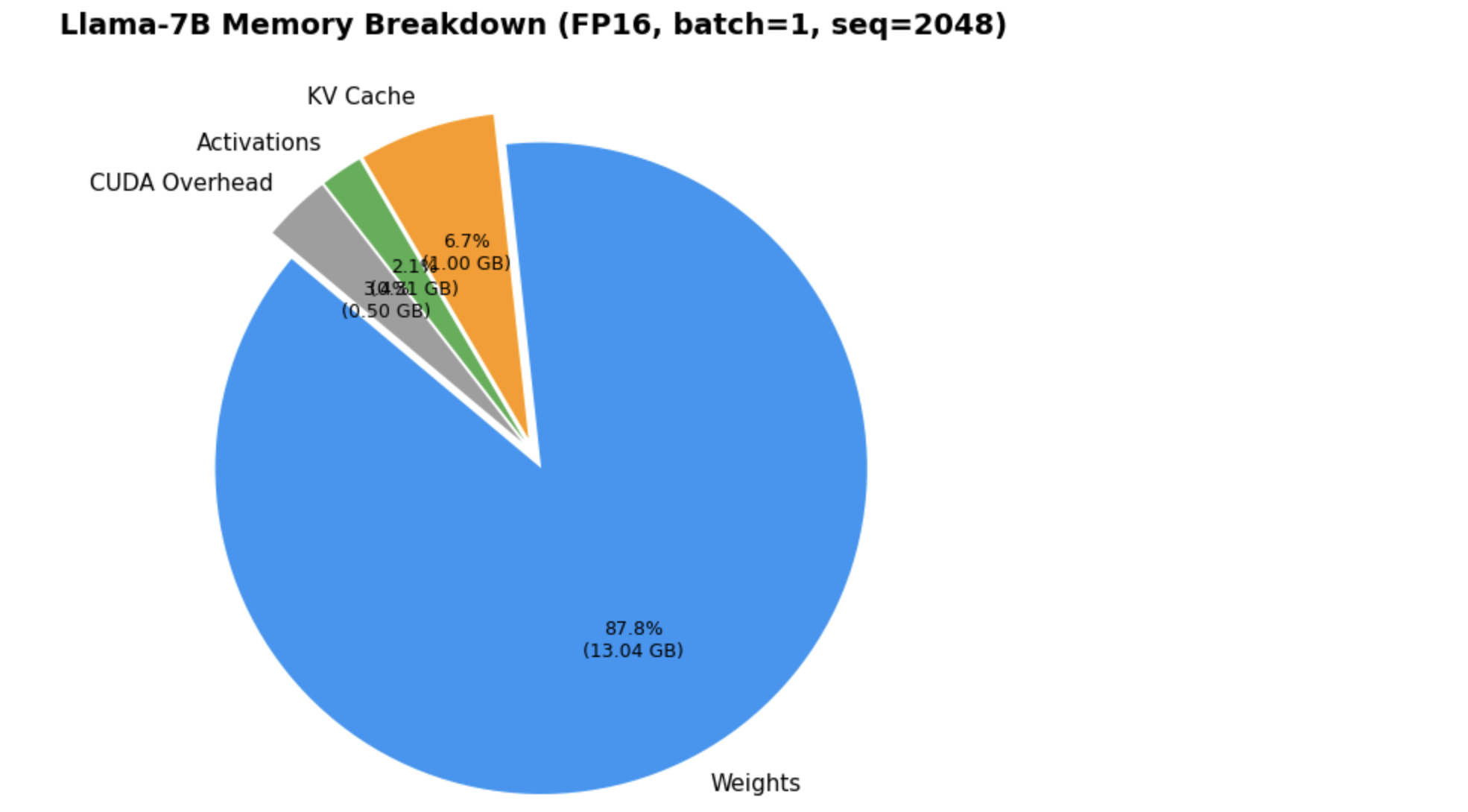
- At batch=1, model weights dominate total memory (~90%+)
- KV cache is small at batch=1 but grows linearly with batch size and sequence length
- Activations during inference are negligible (only one layer active at a time)
- CUDA overhead is a fixed ~0.5 GB cost
Does Llama-70B Fit on A100-80GB?
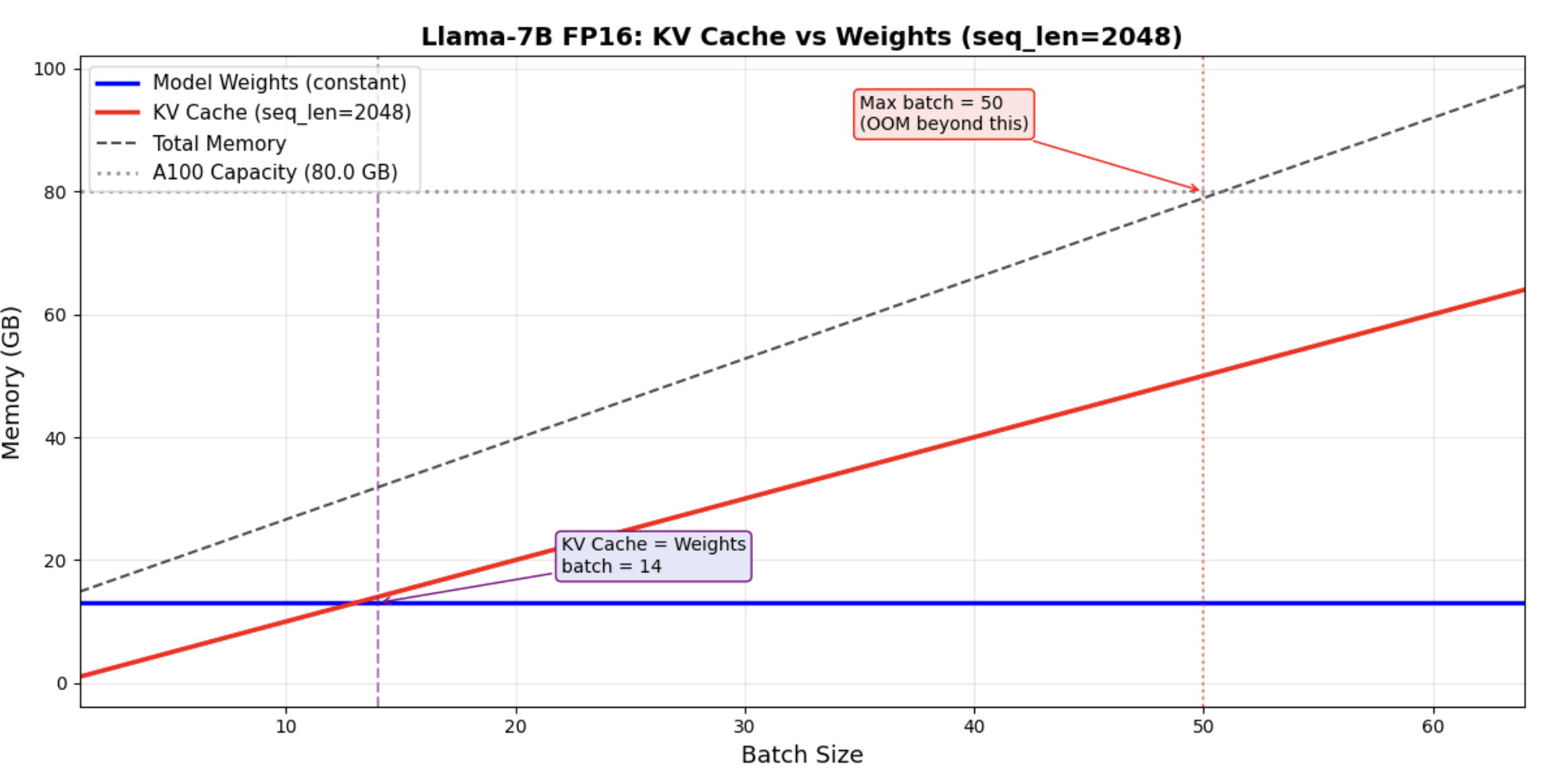
When Does KV Cache Dominate?
At batch=1, weights dominate. But at production batch sizes, KV cache quickly overtakes weights. This plot shows the crossover point for Llama-7B.
Memory Across Model Sizes and Precisions
Key observations:
- Weights scale linearly with parameter count and inversely with quantization.
- INT4 gives a 4x reduction in weight memory vs FP16, making 70B feasible on one GPU.
- KV cache for 70B is smaller than expected thanks to GQA (8 KV heads vs 64 query heads).
- At batch=1, weights dominate. At production batch sizes (32+), KV cache dominates.
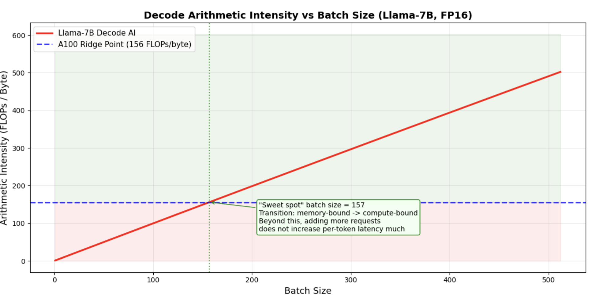
Arithmetic Intensity Analysis
Let's see how arithmetic intensity changes with different operating conditions, and how that determines whether we're memory-bound or compute-bound.
Decode AI vs Batch Size
Decode at batch=1 has an arithmetic intensity of just 1 , only 0.6% of the ridge point. Even at batch=64, we're still deeply memory-bound. It takes a batch size of ~156 to fully saturate the A100's compute capability during decode.
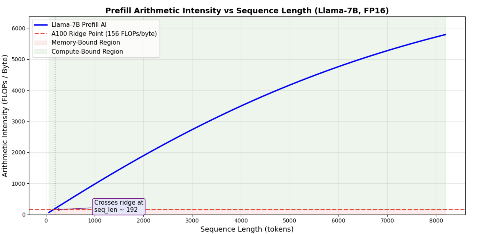
Prefill AI vs Sequence Length
Prefill crosses the ridge point at relatively short sequence lengths (~300-400 tokens). For typical prompt lengths (1K+ tokens), prefill is solidly compute-bound , the GPU cores become the bottleneck, not memory bandwidth.
Time Estimates
Using the roofline model, we can estimate latencies for prefill (TTFT = time to first token) and decode (per-token generation time). These back-of-the-envelope calculations are exactly the kind of reasoning expected in interviews.
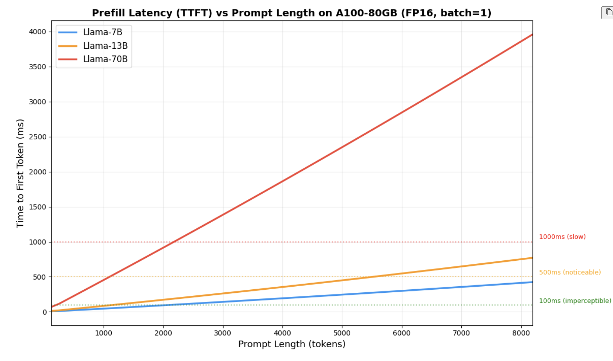
Prefill Latency (TTFT)
Prefill latency scales roughly linearly with prompt length. For Llama-7B on A100, a 2048-token prompt takes about 9 ms , fast enough to be imperceptible.
Decode Latency and Throughput
Decode time stays ~7 ms per step while memory-bound (batch < ~164); total tokens/sec scales with batch. Past the ridge, latency rises and throughput plateaus (~22K tokens/sec). See the diagram below.
The key insight: decode time per step stays nearly constant as batch size increases (while memory-bound). This means total throughput scales linearly with batch size , for free! This is the fundamental insight behind continuous batching.
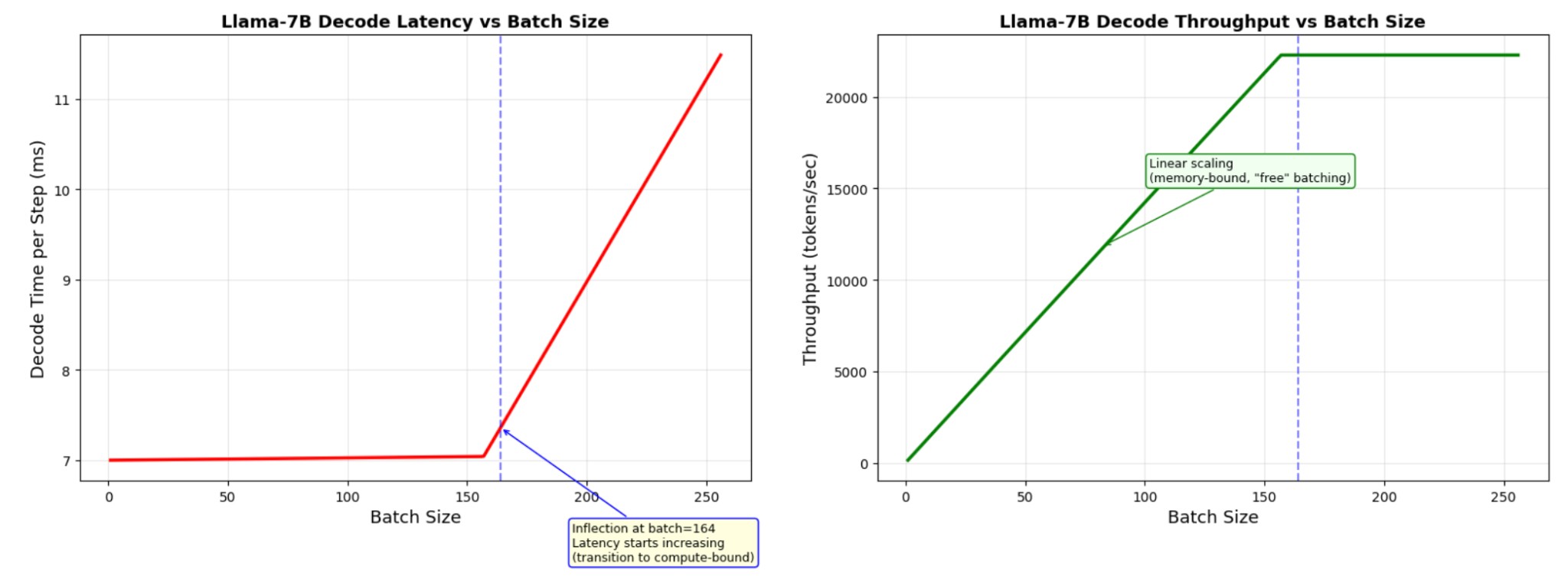
- Decode time per step stays nearly constant as batch size increases (while memory-bound)
- Total throughput (tokens/sec) scales linearly with batch size , for free
- This is the fundamental insight behind continuous batching (vLLM, TGI)
- Per-request latency stays the same , everyone gets the same speed, but the server handles more requests
Key Takeaways
5 Things You Should Know
- "Autoregressive decode is memory-bandwidth-bound, not compute-bound." Each decode step requires reading all model weights from HBM to generate a single token. The arithmetic intensity is ~1 FLOP/byte (at batch=1, FP16), far below the A100's ridge point of 156. This means the Tensor Cores sit idle ~99% of the time during decode.
-
"Prefill is compute-bound for reasonable sequence lengths."
During prefill, the same weights are reused across all tokens in the prompt, giving arithmetic
intensity that scales with
seq_len. For seq_len > ~300 on A100, prefill becomes compute-bound. - "Batching is the primary lever for decode throughput." Since decode is memory-bound, adding more sequences to a batch reuses the same weight data already being streamed from HBM. The per-step latency barely changes, but throughput scales linearly. This is why continuous batching (vLLM, TGI) is transformative.
- "KV cache memory grows as O(batch_size × seq_len × num_layers × d_head × num_kv_heads)." At production batch sizes (32+), KV cache can dominate total GPU memory. This is why PagedAttention, GQA (grouped-query attention), and KV cache quantization are critical.
- "Quantization helps decode more than prefill." Since decode is memory-bound, reducing the number of bytes per weight (FP16 → INT4 = 4x fewer bytes) directly translates to ~4x faster decode. For prefill (compute-bound), quantization helps less unless it also reduces the compute cost.
Quick-Reference Formulas
Keep these formulas in your head for back-of-the-envelope calculations: