A Guide to Fine-tuning Methods in LLMs (Part 1)

Mar 17th, 2025 · 20 min read

This blog explores various fine-tuning methods for Large Language Models. For a better understanding of the motivation behind these techniques, I recommend first reading my article on Memory Optimization in Deep Learning.

Understanding Fine-tuning vs Training

Key Distinction: Training involves starting with random weights, while fine-tuning starts with pre-trained model weights. This fundamental difference shapes our approach to model adaptation.

The Memory Challenge

When running large models on available hardware, you typically have two main options:

Options for Running Large Models:

1. Reduce Memory Footprint
   • Quantization
   • Parameter-efficient methods
   • Gradient checkpointing

2. Distribute Computation
   • CPU offloading with DeepSpeed
   • Model parallelism
   • Pipeline parallelism

Evolution of Fine-tuning Approaches

1. Full Fine-tuning

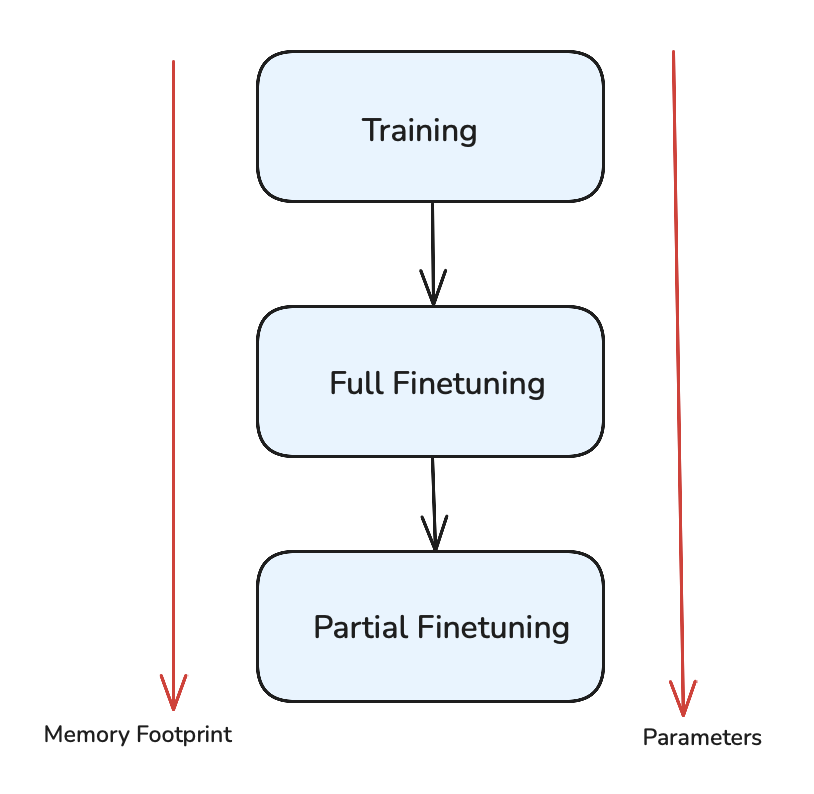
Figure 1: Traditional full fine-tuning approach where all model parameters are updated

In the early days of deep learning, when models had fewer parameters, full fine-tuning was the standard approach. This method updates all model weights during the adaptation process.

2. Partial Fine-tuning

As models grew larger, researchers began experimenting with partial fine-tuning, freezing about 10% of the model weights. While this reduced memory footprint, the performance benefits were limited. Meaningful improvements typically required fine-tuning at least 30% of the model parameters.

The critical question emerged: Could we achieve significant performance improvements while updating only a tiny fraction of parameters? This led to the development of Parameter-Efficient Fine-Tuning (PEFT) methods.

Parameter-Efficient Fine-Tuning (PEFT)

The core idea behind PEFT is strategic: introduce small trainable neural networks called "adapters" at carefully selected locations within the model. These adapters act as learnable interfaces between the model's frozen layers. During fine-tuning, the original pre-trained weights remain unchanged, and only these adapter parameters are updated, making the process highly efficient.

Advantages

Parameter Efficient: Requires only a small fraction of trainable parameters
Sample Efficient: Needs fewer examples for effective fine-tuning
Memory Efficient: Significantly reduced memory footprint

Limitations

Increased Inference Latency: Additional computation overhead during forward pass
Architecture Modifications: Requires changes to model structure

Figure 2: Overview of Parameter-Efficient Fine-Tuning approaches

Understanding Prompt-Based Methods

Hard Prompting

 Example of Hard Prompting:
 
 Input: "How to make a delicious pizza?"
 
 Hard Prompt: "As an expert chef, provide step-by-step instructions for making a delicious pizza:"
 
 This is a discrete text prompt that guides the model's behavior but cannot be optimized during training.

Soft Prompting

 Soft Prompt Example:
 
 Instead of discrete text, we use trainable embeddings:
 [0.23, -0.45, 0.89, ...] → Trained to represent "summarize"
 [0.67, 0.12, -0.34, ...] → Trained to represent "explain"
 
 These continuous vectors are learned during fine-tuning to optimize task performance.

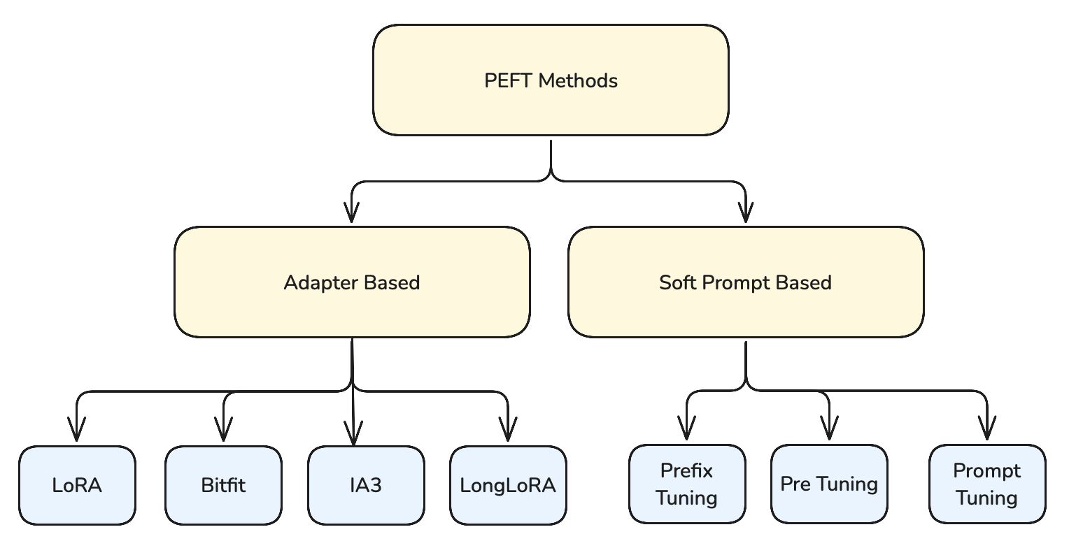
Key Prompt-Based Methods

Prefix Tuning: Adds trainable continuous tokens before specific layers
Prompt Tuning: Prepends trainable embeddings to the input
P-Tuning: Introduces trainable prompts at multiple positions

Understanding Soft Prompts:

Think of soft prompts as the model learning a "language" of its own. For example, when fine-tuned on summarization tasks, the soft prompts might encode patterns that help the model recognize key information and generate concise outputs. While we can't "read" these embeddings directly, their effect on the model's behavior is measurable and consistent.

While these prompt-based methods showed promise, they haven't gained as much widespread adoption as more recent approaches like LoRA, which offers better efficiency and easier implementation.

Understanding SVD and Low-Rank Decomposition

Before diving into LoRA, let's understand the key concept behind it: low-rank matrix decomposition. Through a practical example using SVD (Singular Value Decomposition), we'll see how a large matrix can be represented using fewer parameters. This same principle is what makes LoRA efficient - it essentially adds a low-rank update (product of two smaller matrices) to the original weight matrix.

  # First, let's create a rank-deficient matrix
  import torch 
  import numpy as np
  _ = torch.manual_seed(0)
  
  # Generate a rank deficient matrix W
  d, k = 10, 10
  r = 2  # we are defining a low rank
  W = torch.randn(d, r) @ torch.randn(r, k)  # (10 * 2) * (2 * 10) = (10 * 10)
  print(W)
          

tensor([[-1.0797, 0.5545, 0.8058, -0.7140, -0.1518, 1.0773, 2.3690, 0.8486, -1.1825, -3.2632], [-0.3303, 0.2283, 0.4145, -0.1924, -0.0215, 0.3276, 0.7926, 0.2233, -0.3422, -0.9614], [-0.5256, 0.9864, 2.4447, -0.0290, 0.2305, 0.5000, 1.9831, -0.0311, -0.3369, -1.1376], [ 0.7900, -1.1336, -2.6746, 0.1988, -0.1982, -0.7634, -2.5763, -0.1696, 0.6227, 1.9294], [ 0.1258, 0.1458, 0.5090, 0.1768, 0.1071, -0.1327, -0.0323, -0.2294, 0.2079, 0.5128], [ 0.7697, 0.0050, 0.5725, 0.6870, 0.2783, -0.7818, -1.2253, -0.8533, 0.9765, 2.5786], [ 1.4157, -0.7814, -1.2121, 0.9120, 0.1760, -1.4108, -3.1692, -1.0791, 1.5325, 4.2447], [-0.0119, 0.6050, 1.7245, 0.2584, 0.2528, -0.0086, 0.7198, -0.3620, 0.1865, 0.3410], [ 1.0485, -0.6394, -1.0715, 0.6485, 0.1046, -1.0427, -2.4174, -0.7615, 1.1147, 3.1054], [ 0.9088, 0.1936, 1.2136, 0.8946, 0.4084, -0.9295, -1.2294, -1.1239, 1.2155, 3.1628]])

  # Let's verify the rank of our matrix
  W_rank = np.linalg.matrix_rank(W)
  print(f'The Rank of Matrix is: {W_rank}')
        

The Rank of Matrix is: 2

As expected, the matrix has rank 2, confirming that all its information can be represented using just two dimensions, despite being a 10×10 matrix. This is a key insight into why low-rank methods work.

 # Performing SVD on W (U * S * V^T)
 U, S, V = torch.svd(W)
 
 U_r = U[:, :W_rank]
 S_r = torch.diag(S[:W_rank])
 V_r = V[:, :W_rank].t()
 
 A = U_r @ S_r
 B = V_r
 
 print(A.shape, B.shape)
        

torch.Size([10, 2]) torch.Size([2, 10])

SVD decomposes our matrix into three components, but remarkably, we only need to keep the first two singular values and their corresponding vectors. This is because these capture the essential structure of our matrix, while the remaining values are effectively zero.

 # Let's verify our decomposition works perfectly
 bias = torch.randn(d)
 x = torch.randn(d)
 y = W @ x + bias
 y_hat = (A @ B) @ x + bias
 
 print(f'Values with Original Weights: {y}\n\n')
 print(f'Values with (A * B) Weights: {y_hat}')
        

Values with Original Weights: tensor([-2.1548, 0.4832, 1.2947, -0.8374, 0.3158, 1.0483, 2.3690, 0.8486]) Values with (A * B) Weights: tensor([-2.1548, 0.4832, 1.2947, -0.8374, 0.3158, 1.0483, 2.3690, 0.8486])

This example demonstrates the power of low-rank decomposition: we could perfectly replicate the behavior of the original weights using far fewer parameters. A and B combined have only 40 parameters (10×2 + 2×10 = 40), while the original W matrix had 100 parameters (10×10 = 100). This 60% reduction in parameters is exactly the kind of efficiency that makes LoRA so powerful.

Low-Rank Adaptation (LoRA)

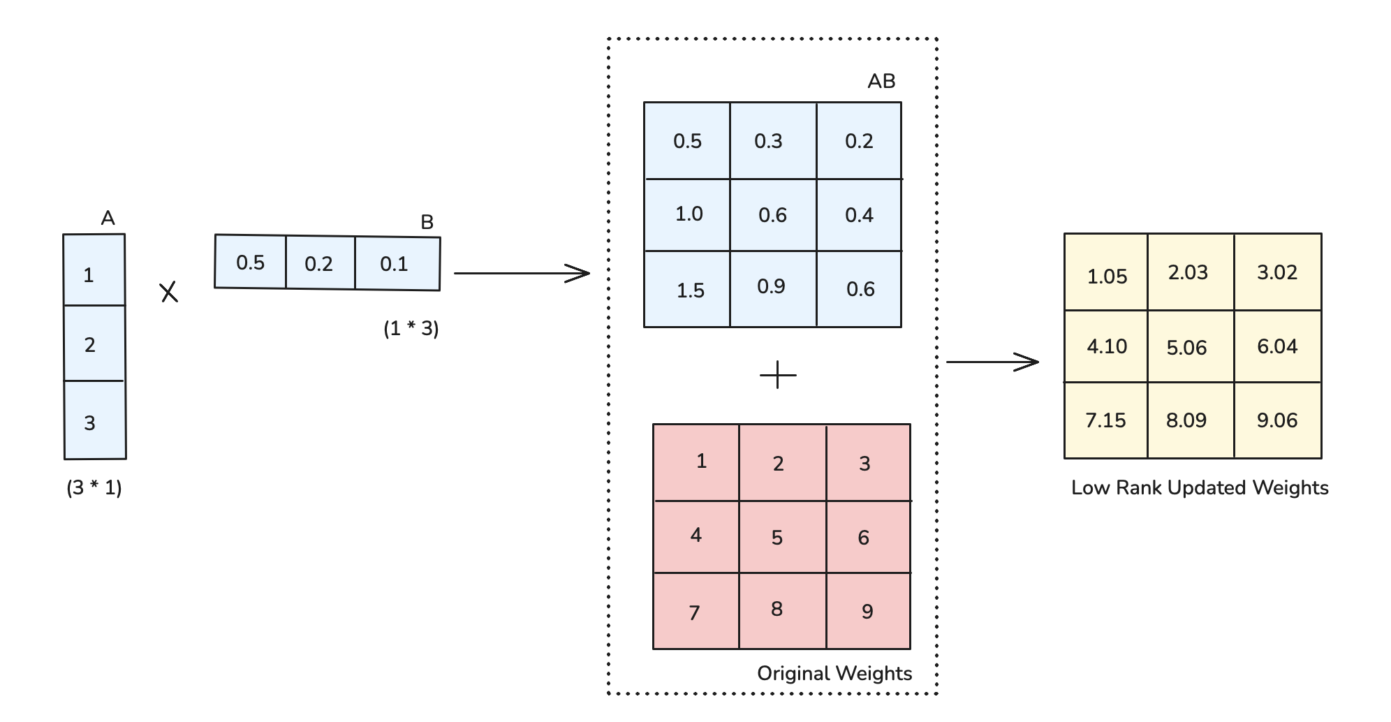
The main idea of Low-Rank Adaptation (LoRA) is to decompose weight updates into low-rank matrices, train these smaller matrices, and then add their product back to the original weights.

Let's break down how LoRA works: Instead of directly updating the large weight matrices of the model, LoRA introduces two smaller matrices (A and B) whose product approximates the weight update. This approach significantly reduces the number of trainable parameters while maintaining model quality.

Figure 3: LoRA's low-rank matrix decomposition and update process

 Mathematical Formulation of LoRA:
 
 Instead of learning the full weight update ΔW, LoRA decomposes it as:
 ΔW = α(A × B)    // where α is the scaling factor (in our example, α = 1)
 // α determines how much weight to give to the LoRA update
 
 where:
 From the diagram example:
 • A is a matrix of shape (3 × 1): [1, 2, 3]
 • B is a matrix of shape (1 × 3): [0.5, 0.2, 0.1]
 • r = 1 (rank of decomposition)
  
 Final Weight Update:
 W = W₀ + ΔW
 where W₀ is the original weight matrix [1,2,3; 4,5,6; 7,8,9]
 
 Key Insight: With just 6 trainable parameters (3 in A + 3 in B),
 we can update a 3×3 matrix containing 9 weights!
        

Key Advantages of LoRA

Unlike traditional adapter methods that add extra layers and increase inference latency, LoRA's design offers a unique advantage: the trained matrices can be merged with the original weights at inference time, resulting in zero additional latency.

Serving LoRA Models

One of LoRA's most powerful features is its flexibility during inference. There are two main approaches:

Merged Weights

Add LoRA updates (A×B) back to original weights
Zero inference overhead
Same memory footprint as original model
Best for single-task deployment

Separate Weights

Keep LoRA matrices separate
Switch between different fine-tuned versions
Combine multiple LoRA adaptations
Ideal for multi-task scenarios

This flexibility allows for interesting deployment scenarios. For example, you could have a base model with different LoRA adaptations for different languages or tasks, and dynamically choose or even combine them at inference time.

Figure 4: Different approaches to serving LoRA models - merged vs separate weights

Storage Benefits of Separate LoRA Weights: A Simple Example

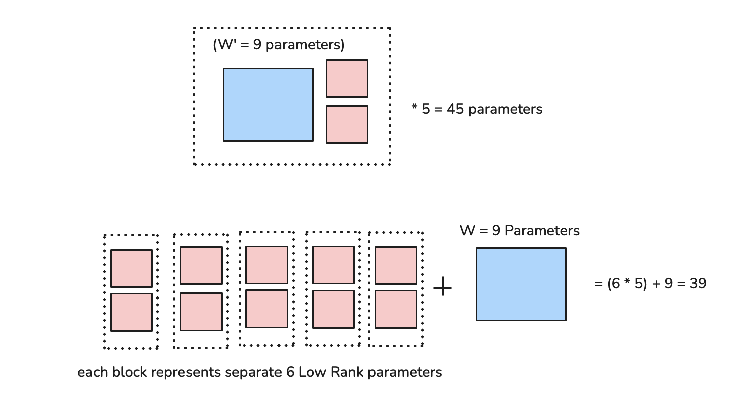
Let's say we have a small weight matrix W of size 3×3 (9 parameters) and 5 different customers:

Option 1 (Merged Weights): • Store 5 full matrices (Wʹ) of size 3×3 • Total storage: 9 parameters × 5 = 45 parameters

Option 2 (Separate LoRA): • Store 1 base matrix W (9 parameters) • Store 5 sets of LoRA matrices A(3×1) and B(1×3) • Each LoRA pair needs 6 parameters (3 + 3) • Total storage: 9 + (6 × 5) = 39 parameters

Even in this tiny example, separate storage saves ~13% space. The savings become much more dramatic with real-world model sizes and more customers.

QLoRA: Quantized LoRA

QLoRA combines the efficiency of LoRA with the memory benefits of quantization. It's a powerful approach that makes fine-tuning possible on consumer GPUs while maintaining model quality.

Key Components

Base model weights are frozen and quantized (typically to 4-bit)
LoRA parameters remain in full precision (16-bit)
Gradients computed in full precision during backpropagation

Why This Works

Most memory is in frozen weights - safe to quantize
LoRA updates need precision for learning - kept in 16-bit
Dequantization during forward pass preserves accuracy

Thanks for sticking till the end! In Part 2, we'll explore advanced topics including model merging and multitask fine-tuning. Stay tuned!